While we have several ways for computing good linearizations for a cluster from scratch, sometimes we don’t start from scratch. We may have our own linearization already, but receive (through so far unspecified means) another linearization from a peer. If it’s strictly better, we could just switch to it. But what if our linearization is better in some places, and theirs is better in other places? Can we somehow combine the “smarts” that they’re based on, to construct an even better linearization?
As a reminder, we compare linearizations by computing all cumulative (size, fee) points after every chunk, and connecting them by straight lines. Each linearization has such a segmented line, which we call the fee-size diagram. If a linearization A has a diagram that is nowhere below that of linearization B, and at least in some places above it, we say A is strictly better than B. If the diagrams coincide everywhere, they’re equal. If one diagram is on top in some place(s) and the other is on top in others, we call them incomparable.
Due to the (so far unproven, but accepted EDIT: now proven, thanks to this thread) property that every cluster has a well-defined non-empty set of optimal linearizations (which are all equal to each other, and all strictly better than all other linearizations), it must be the case that if two incomparable linearizations exist, there must exist at least one linearization that’s strictly better than both. This topic is about finding such combined linearizations.
Algorithms
Best-chunk merging
We’ve known a simple merging algorithm for a while:
Given two linearizations L1 and L2:
While not all transactions have been processed:
Find highest-feerate prefix P1 among all unprocessed transactions in L1.
Find highest-feerate prefix P2 among all unprocessed transactions in L2.
Include the transactions from the higher-feerate of P1 and P2 in output linearization.
Mark the included transactions as processed
This algorithm can have \mathcal{O}(n^2) runtime in the number of transactions, because there can be n iterations, and each can require \mathcal{O}(n) work to find the highest-feerate prefix. In \mathcal{O}(n) time we can of course also compute the full chunking of L1 and L2 (rather than just the first chunk), and it may be possible to reuse part of that computation across iterations; that may enable a lower complexity, but it seems nontrivial. And given the fact that in every case we’ll probably want to run at least an ancestor-set based linearization from scratch ourselves (which is also \mathcal{O}(n^2)), it’s probably fine to target the same complexity for a merging algorithm.
Sadly, this algorithm doesn’t always produce an output that’s better or equal than both inputs. It will produce a linearization whose diagram is at no point below the lowest of the two input diagrams, but that’s not a particularly high bar. We could instead just stick with either one of the inputs instead to achieve that level of quality. In typical cases it’ll be better of course, but there are no guarantees. And it is easy to find examples where the result is just one of the inputs, and thus still incomparable to the other one.
The first input linearization is the ancestor set sort: [B,F,A,D,E,C], which is chunked as [BFADE,C].
The second input is [B,A,E,C,D,F], which is chunked as [BAECD,F]. The BAECD chunk has higher feerate (18/7=2.571) than BFADE (23/9=2.556), but during the F part it is overtaken by BFADE.
The result of merging is just the second input again.
The optimal linearization would be [B,A,D,E,F,C], chunked as [BADE,F,C].
What we observe is that there is actually a common subset (BADE) of the two initial chunks that can be moved to the front, but the merging algorithm does not consider this.
Intersection merging
In an attempt to address that, let’s add a step to the merging algorithm to consider intersections:
Given two linearizations L1 and L2:
While not all transactions have been processed:
Find highest-feerate prefix P1 among all unprocessed transactions in L1.
Find highest-feerate prefix P2 among all unprocessed transactions in L2.
Let P3 be the intersection of P1 and P2. This is necessarily topologically valid.
Include the transactions from the highest-feerate of P1, P2, and P3 in output linearization.
Mark the included transactions as processed
While it adds a step, the complexity is unchanged. Unfortunately, it still doesn’t always result in a better linearization:
The first input linearization is the ancestor set sort: [B,A,E,D,G,C,F], which is chunked as [B,AEDGC,F].
The second input is [B,A,C,F,E,D,G], which is chunked as [BACFE,DG]. The BACFE chunk has higher feerate (66/5=13.5) than B (13) initially, but gets overtaken by the AEDGC chunk.
The result of merging is equal to the second input.
The optimal linearization would be [B,A,C,E,D,G,F], chunked as [BACE,DG,F].
Again the crux is discovering an intersection (BACE), but this time between the BACFE chunk and not one but two chunks of the other input (B and AEDGC).
Prefix-intersection merging
The solution is to attempt more intersections. Observe that a linearization is really a way of constraining the search for subsets to just prefixes of the linearization. Given the intuition gained above that incomparabilities always seem to be due to a non-considered intersection between the two linearizations, it seems worthwhile try all intersections between prefixes of the first with prefixes of the second linearization. There can be a quadratic number of such intersections however, but maybe we can limit ourselves to just intersections that involve the best chunk of one of both linearizations at least:
Given two linearizations L1 and L2:
While not all transactions have been processed:
Find highest-feerate prefix P1 among all unprocessed transactions in L1.
Find highest-feerate prefix P2 among all unprocessed transactions in L2.
Find the highest-feerate set among all these:
Intersections between P1 and all prefixes of L2.
Intersections between P2 and all prefixes of L1.
Include the transactions from that set in the output linearization.
Mark the included transactions as processed
The various intersections between P1 and prefixes of L2 can be computed incrementally (keep adding transactions from L2 if they’re in P1, and remember the best one), and similarly for P2 with prefixes of L1. This, like finding the Pi in the first place, can be done in \mathcal{O}(n) time. The result is still an \mathcal{O}(n^2) algorithm.
Surprisingly, this algorithm seems powerful enough to always find a linearization that’s strictly better than both inputs if they’re incomparable (and at least as good as the best of the two if they are comparable). This works regardless of the quality of the input linearizations (e.g. they don’t need to be ancestor sort or better), and does not require connected chunks (see linearization post-processing). No proof, though.
Update: simpler and proven merging
See the discussion further in this thread (thanks, @ajtowns).
It appears that it suffices to only consider the intersections between the higher-feerate out of P_1 and P_2, with all prefixes of the linearization of the other input:
Given two linearizations L_1 and L_2:
While not all transactions have been processed:
Find highest-feerate prefix P1 among all unprocessed transactions in L1.
Find highest-feerate prefix P2 among all unprocessed transactions in L2.
If P_1 has lower feerate than P_2, swap P_1 with P_2 and L_1 with L_2.
Find the highest-feerate set among all intersections between P_1 and the prefixes of L_1.
Include the transactions from that set in the output linearization.
Mark the included transactions as processed
Instead of describing the resulting set as an intersection, it can also be seen as the highest-feerate prefix of P_2, reordered according to the order these transactions have in L_1.
A proof for this scheme can be found in this thread.
One way of characterising a chunk is by listing its childless-descendants; for BACFE, those would be E and F. But in this case F’s feerate alone is 11, while BACFE’s is 13.2; which gives you an easy clue that splitting that chunk into [BACE,F] would be an improvement.
I think you could extend this comparison to create a compatible total order just by saying “given two diagrams, d_1 and d_2, then if x_0 is the earliest point where d_1(x_0) \ne d_2(x_0), then d_1 > d_2 iff d_1(x_0) > d_2(x_0)” ?
I think “prefix-intersection merging” then guarantees to produce a linearisation L_3 such that L_3 \ge L_1 and L_3 \ge L_2 according to that total order. I don’t think it guarantees that L_3 will be comparable to L_1 or L_2 according to the original partial order, but I think you’d need a fairly complicated cluster for that to actually occur.
Prefix-intersection merging on L_1 and L_2 gives a linearization L_3 such that L_3 \geq L_1 and L_3 \geq L_2, according to the usual preorder on linearizations. If additionally L_1 and L_2 were incomparable (i.e., L_1 \ngeq L_2 and L_1 \nleq L_2), then L_3 > L_1 and L_3> L_2.
No proof, but I’ve spent a decent amount of CPU time (weeks) on trying to find counterexamples.
Under your total ordering it holds for any of these merge algorithms (including best chunk merging) that L_3 \geq L_1 and L_3 \geq L_2. The surprising part is that prefix-intersection merging seems powerful enough to achieve that under the preorder.
I haven’t processed this whole post yet, but just wanted to add an aside/reminder for the sake of our intuition: even if a linearization is strictly better than another one, it may still be the case that merging the two (even using our most naive algorithm) would produce a linearization better than either.
Right, the childless-descendants in an optimal chunk are always higher feerate than the chunk itself (or more generally, any “bottom” subset (a subset that includes all its descendants) must have higher feerate than the chunk itself - if not, that subset could be removed without breaking topology, and doing so would increase the feerate).
This could be the basis for another general post-processing step (e.g. try all bottom subsets of 1 or 2 transactions, and if they have lower or equal feerate than the overall chunk, split them up). Similarly for top transactions with higher or equal feerate than the overall chunk. Of course, we could also hope to build linearization algorithms that just don’t give rise to such chunkings in the first place.
FWIW, I think that relaying the set of childless-descendants for each chunk to a peer is another hypothetical way of conveying knowledge of linearizations. It could be made Erlay-compatible as it has set semantics, and with that set one can reconstruct the same linearization (and likely gives a decent result even if the clusters don’t exactly match).
Yes, absolutely. I’ve changed the text to say “could” instead of “should”. I think we’ll want to run prefix-intersection merging (or some further iteration of this idea) anytime we have distinct linearizations of the same transactions. It even works when the input linearizations don’t cover the exact same transactions but there is some overlap, though I haven’t run tests for that.
I’ve now learned that our comparison operation on linearizations (through comparing the diagram) is not a partial order but a preorder. The difference is that distinct elements can be equivalent under a preorder.
By moving a subset of transactions, whose combined feerate is S, to the front of a linearization whose first chunk has feerate <= S, while keeping the relative order within the moved and within the non-moved transactions the same, the feerate diagram will be >= the old one (obviously subject to that being topologically valid).
If so, I may be able to prove prefix-intersection merging always results in something >= both original linearizations.
I think you need slightly different terminology: given an ordered set of transactions T = t_1, t_2, .., t_n then Chunk(T) splits up that list, eg C_1 = t_1, t_2; C_2 = t_3; C_3 = t_4, .., t_n while maintaining its order (T = \sum Chunk(T)), and gives you a valid diagram (s(C_1) \ge s(C_2) \ge s(C_3)). Then if chunking a given ordering of txs results in a single chunk, ie Chunk(T) = C, then any reordering of T will result in a comparable diagram that is equal to or better than the diagram for T.
(That’s then obviously true because the diagram has the same start/end points, the first diagram for T is just a line, and the chunking inequality ensures the diagrams are concave)
Assume you have a function C(L) that takes a linearisation L and splits that into P_L, T_L where P_L is the first chunk, and T_L is the rest of the linearisation. If L is non-empty, P_L is non-empty also; however T_L may be empty.
Assume you can calculate L - X where L and X and the result is just L with the transactions in X removed
We say that A \le B by doing a feerate diagram comparison and noting B is has a higher or equal feerate at all points.
I think prefix-intersection merging, M(L_1, L_2) is equivalent to:
Take P_1, T_1 = C(L_1) and P_2, T_2 = C(L_2)
Reorder the transactions in P_1 to match the order they appear in L_2, call this P^\prime_1, and then calculate R_1, X_1 = C(P^\prime_1). Note that P_1 \le R_1.
Calculate R_2, X_2 in the same way from P_2.
Choose the highest feerate chunk from R_1, R_2:
If R_1 is the highest, then: M(L_1, L_2) = R_1 + M(X_1 + T_1, L_2-R_1)
For the case where R_1 is highest, then M(L_1, L_2) = M(R_1 + X_1 + T_1, L_2) and L_1 \le R_1 + X_1 + T_1.
The question is whether L_2 \le R_1 + (L_2-R_1), noting that the transactions in R_1 that we’ve removed from L_2 maintain their order, and have an equal or higher feerate than the original best chunk.
Consider each chunk from L_2, call them c_1, c_2, c_3, \dots, c_n. Then define d_i = c_i - R_1, and e_i = c_i - d_i. In that case R_1 = e_1 + e_2 + e_3 + \dots + e_n (because R_1 is the first chunk of P^\prime_1 which had its transactions put in the same order as L_2).
We see L_2 = \gamma_n, and R_1 + (L_2 - R_1) = \epsilon_n + \delta_n and \epsilon_n = \epsilon_j + \zeta_j. Note that the feerate of \zeta_j is greater or equal to the feerate of R_1 = \epsilon_n in all cases – otherwise those transactions would not have been included in R_1 when calculating the chunk.
Consider total size of \gamma_j, S(\gamma_j) and its total fee F(\gamma_j). Note that the feerate diagram of L_2 is made up of the pairs S(\gamma_j), F(\gamma_j).
If we consider \epsilon_j + \delta_j then we simply have S(\epsilon_j + \delta_j) = S(\gamma_j) and F(\epsilon_j + \delta_j) = F(\gamma_j).
Now consider \epsilon_j + \delta_j + \zeta_j – for which the feerate diagram at position S(\gamma_j) is at least F(\epsilon_j + \delta_j), ie at least F(\gamma_j). But we know \zeta_j has a higher fee rate than any chunk in \epsilon_j + \delta_j, so the feerate diagram of \epsilon_j + \zeta_j + \delta_j is an improvement. That gives \gamma_j \le \epsilon_n + \delta_j, and choosing j=n gives L_2 = \gamma_j \le \epsilon_n + \delta_n = R_1 + (L_2 - R_1). QED?
Why? Moving part of P_1 to the front could put a higher feerate new chunk up front.
M_{PI}(L_1,L_2)
What is PI?
FWIW, my (incomplete) proof sketch is as follows:
Assume that the following holds: moving transactions to the front of a linearization such that they form a new chunk, while leaving the internal ordering within moved and non-moved transactions the same, is a non-worsening of the diagram if the new chunk’s feerate is >= the original first chunk’s feerate. (no proof EDIT: see proof here)
Also assume that reordering the transaction within one chunk can never worsen the diagram (worst case the chunk set remains the same, best case it splits in multiple parts).
The prefix-intersection merging algorithm can be seen as starting with two linearizations L_1 and L_2, and in each step moves some transactions to the front of both. Each step is a non-worsening of the diagram of both, and in the end, both linearizations are identical. That resulting linearization is thus better or equal than each of the inputs. To see why each step is a non-worsening:
WLOG, assume the intersection found is a subset of L_1's first chunk, in the order of transactions of L_2. (swap the linearizations if not)
The change applied to L_1 is just a reordering of its first chunk, which is fine.
The change applied to L_2 is moving a new chunk to the front, of feerate at least that of its original first chunk (if not, that chunk would have been chosen instead), leaving the order within moved and non-moved transactions the same. This is fine.
Afterwards, both linearizations start with the same transactions (at least one, so progress is made), so we can continue with just the distinct suffix.
Interesting observation, I hadn’t realized this before: any suffix of a chunk’s linearization (which leaves at least one transaction off) must have higher feerate than the chunk itself. If it didn’t, the chunk without the suffix would have higher feerate and thus be the chunk instead.
yeah, chunking means that suffix-pays-for-prefix. (could be equal rather than higher, depending on whether chunking is maximal or minimal) [edit: i guess we always want minimal – as if we have two chunks of the same feerate, it’s easy to combine them when building a block, but much harder to split a chunk]
This \epsilon_j + \delta_j + \zeta_j diagram, is that considering this expression at different values of j? I’m confused how it can be evaluated at S(\gamma_j), or really how it forms a diagram at all.
Also generally, to prove a diagram is everywhere ≥ than another, you need to show both that all points of the first lie ≥ the second, but also that all points of the second lie ≤ the first.
(I’m finding it hard to work out a decent way of comparing diagrams that doesn’t get lost in details really quickly. Perhaps the problem is that I really only want to compare orderings of a given set of transactions after chunking them, not compare two orderings of potentially two different sets of transactions with arbitrary groupings)
Anyway, I guess the general case I’m going for here is
\epsilon_n + \delta_j \ge \gamma_j + \zeta_j
Those are comprised of the exact same txs, ie d_1, .., d_j and e_1, .., e_n, but in different orders. The QED step is setting j=n giving \zeta_j=\emptyset, and thus R_1 + (L_2 - R_1) = \epsilon_n + \delta_n \ge \gamma_n = L_2. \ge is a diagram comparison after chunking the txs, and +, \sum are concatenation.
The initial step for j=0 is easy: \delta_0 = \gamma_0 = \emptyset and \epsilon_n = \zeta_0 by construction.
The inductive step is to show \epsilon_n + \delta_{j+1} \ge \gamma_{j+1} + \zeta_{j+1}. To show that, we have:
Ok, I’m with you. I didn’t realize before that + meant concatenation.
So you’re essentially relying on 3 steps which each individually don’t make the diagram worse, and composing them to show that moving a new higher-fee chunk to the front while leaving internal ordering the same, makes the overal thing not worse.
Those 3 steps are:
If a \geq b, then a + c \geq b + c. That seems reasonable, though I do want to think through what happens when c gets chunked together with some suffix of a or b (but not both).
Two chunks can be swapped if the second one has higher feerate than the (highest chunk feerate in) the first. That’s probably true under some conditions, but it’s not entirely clear to me what those conditions are. Does this also hold when both/either isn’t really a chunk (in the sense of being chunked togeter) but consists of multiple?
Reordering and splitting a chunk is fine. If it’s really a chunk, then this is obviously the case - it’s just reordering transactions within a chunk which at worst has no effect on the diagram - but is it obvious here that c_{j+1} is actually a single chunk, when considered in the linearization presented there?
In short, I think we need some theorems that relate diagram quality with transformations/reorderings of the linearization, even when those modify chunk bounaries.
I think all these steps rely really heavily on how they’re setup via the prefix intersection algorithm – eg, c_{j+1} is a chunk in \gamma_j + c_{j+1}, because \gamma_j = c_1 + c_2 + .. + c_j and c_1, c_2, .., c_n is a correct chunking, and then the fact that you generate a chunking by merging tx sets in any order means that if you add stuff on the end of that, you can start off with that chunking, and then you’ll only potentially be merging those chunks from the tail, you’ll never need to split them up.
I’m starting to have a bit of luck formalising this in lean4, fwiw, but it’s slow progress : I can convert a list of txs into a chunking, and compare fee rate graphs (evaluating the diagram at each integer byte/weight with a total fee in \mathbb Q), but currently don’t have any theorems about any of that.
(If you have a better way of defining a diagram than as a function from \mathbb N \to \mathbb Q that’d be great. I started off trying to do line segments from (s_1,f_1) \to (s_2,f_2) but that got super painful super fast)
I guess what we need is a slightly more general concept of a chunking, which is a sequence of transaction sets, without the requirement that their feerates are monotonically decreasing.
And we can define a diagram for such a general chunking too, it’s just not necessarily convex concave.
Let C\left((s_1,s_2,\ldots,s_n)\right) = (t_1,t_2,\ldots,t_m) be the chunking operation, which just merges adjacent sets whenever the later one is higher feerate than the earlier one.
Then there are some theorems that hold, I think, such as:
I think diagrams for chunked sets are concave not convex? (I looked it up after I said convex previously – Concave function - Wikipedia – outside of polygons, this terminology always confuses me)
If the “unicity of corresponding chunking” theorem holds (which seems fairly obvious to me, though I lack the formality to prove it), then this also holds:
Oh, this gets easier if you split C into two steps: one to raise List Tx into List (List Tx) (by putting every element in a singleton list), call it c=R(s), and the other that repeatedly merges adjacent chunks when they’re out of order and gives you the best chunking, b=C(c)
Then you have C(a) \ge a fairly straightforwardly (hopefully?), and also C(a+b) = C(C(a) + b) = C(a+C(b)) = C(C(a)+C(b)) directly from merge order independence.
Also, I think that means you’re always comparing chunks (List Tx) by feerate, and chunkings (List (List Tx)) by diagram.
I was thinking of C as an operation on a list of (generalized, not necessarily monotonically decreasing feerate) chunks - whether those are obtained by starting with the singletons from a linearization, or something else.
We want to prove that C(\epsilon_n + \delta_n) \geq \gamma_n I think. I suspect it’s possible to adapt your derivation above to work by placing C() invocations carefully, and using the rules around it.
EDIT: this theorem is insufficient, as it doesn’t allow for cases where the moved good transactions get chunked together with bad transactions; a scenario that is possible in the prefix-intersection merging algorithm.
Theorem
Given the following:
A linearization L
A topologically valid subset T of the transactions in L (which we’ll call “good” transactions).
The good transactions merge into a single chunk of feerate f, when considered in the order they appear in in L.
The highest chunk feerate of the bad transactions, again retaining the order of L, does not exceed f.
Under those conditions, moving the good transactions to the front of the linearization (leaving the internal order of good transactions and that of bad transactions unchanged) results in a better or equivalent linearization (by becoming the new first chunk, of feerate f).
Proof
Observe that, among the set of linearizations for the same transactions which leave the internal orderings unchanged, none can give rise to a chunk feerate exceeding f. If it did, there must be some topologically valid subset v of transactions, consisting of a union of a prefix of the good transactions and a prefix of the bad transactions, whose combined feerate exceeds f. No prefix of the bad transactions can exceed feerate f, thus there must be a prefix of the good transactions that does. This is in contradiction with the given fact that all the good transactions merge into a single chunk of feerate f.
Further observe that all good transactions merging into a single chunk of feerate f implies that any suffix of good transactions has feerate \geq f.
To prove that moving all good transactions to the front of the linearization always results in a better or equivalent linearization as the original, we will show that the following algorithm never worsens the diagram, and terminates when all the good transactions are in front:
Compute the chunking (c_0, c_1, \ldots, c_n) of the current linearization, merging equal-feerate chunks (this does not break the monotonic decrease property, and guarantees each c_i has distinct feerate).
Find the last chunk index t such that c_t \cap T \neq \emptyset.
Modify the linearization by reordering the c_t transactions such that all of c_t \cap T are at the start of c_t.
Repeat (which implies rechunking).
To show that this never worsens the diagram, it suffices to see that reordering transactions within a chunk at worst leaves the chunk unchanged, and at best splits it, which improves the diagram.
Further, this algorithm makes progress as long as c_t does not start with all its good transactions. As long as that is the case, a nonzero amount of progress towards having all the good transactions at the start of the linearization is made. Thus, after a finite number of such steps, that end state must be reached.
It remains to be shown that c_t cannot start with all its good transactions unless the end state is reached. Assume it does start with all its good transactions. The set c_t \cap T is a suffix of the good transactions, and thus has feerate \geq f. Since c_tstarts with c_t \cap T, the chunk c_t itself must have feerate \geq f. However, every chunk must have feerate \leq f. The combination of those two means c_t has exactly feerate f. There can only be one such chunk (as all c_i have distinct feerates), and it must be the first one (because no higher feerate is possible), so t=0. In this case, we are in the end state, because the first chunk is the only one with good transactions, and all good transactions are at its front.
I don’t like that assumption; you can only check it after you’ve done all the work, rather than beforehand, and it conceivably could turn out to be false. I think a better assumption would be “The first chunk of L has a feerate f_0 which does not exceed f”
I think by “topologically valid” you’re meaning that no parents follow their child, and that all parents are included; ie if you have c spends p spends gp, then [gp, p, c] and [gp, p] are topologically valid, but [p,c] is not. This lets you say that if b is topologically valid, then for any a,x, if a + b is topologically valid, then b + a is also topologically valid. You also have a + b being t.v implies a is t.v, and that gives you b_1 + b_2 + .. + b_n being t.v and a_0 + b_1 + .. + b_n + a_n being t.v gives b_1 + .. + b_n + a_0 + .. + a_n being t.v.
For the intermediate steps, you’re not moving txs all the way to the front, though, so I think you want something slightly cleverer still; perhaps a + b + c and a + c being t.v gives a + c + b being t.v is enough.
I think you could rewrite this slightly:
Chunk to (c_0, .., c_n) normally, pick t.
Note that fee rate of c_0 \le f (is it?) and the feerate of c_i \ge c_{i+1} as a property of chunking.
Construct c^\prime_t by reordering c_t to ensure the good txs are at the start.
If c_{t-1} has feerate less than f or c_t \cap T \ne T then the good txs at that start of c^\prime_t will have higher feerate than c_{t-1} (because every tail of T has higher feerate than f) and the final good txs will appear in chunk t-1 or lower on the next round.
Otherwise, the good txs at the start of c^\prime_t are precisely T, those txs and each of c_0, .., c_{t-1} have feerate f (as c_0's feerate is f_0 \le f by assumption, and by feerate c_i \ge c_{i+1} due to the chunking algorithm, and T has feerate f by definition). But in that case reordering to be T, c_0, .., c_{t-1} doesn’t change the diagram, because all the reordered chunks have precisely the same feerate.
Note that your good txs will never get split up once you’ve moved them, so c_0 will have the same composition and feerate it had originally until t=0 and c_0 \cap T = T, and merging some subset of the good txs into c_{t-1} will mean all of them are merged.
Also, I think your theorem needs a tweak: if you have equal size txs with feerates a=0,b=6,c=9,d=0,e=5, and start with L=[a,b,c,d,e] and T=[a,e], then your original chunks were [a,b,c], [d,e] with both those chunks and T having a feerate of 5. But your new linearisation of [a,e,b,c,d] chunks to [a,e,b,c] [d] with feerates 6.25 and 0. Which is fine, it’s just that T doesn’t actually become the first chunk, since we end up finding a chunk with feerate greater than f instead.
It can be checked beforehand: it’s just the feerate of the first chunk of L \setminus T is \leq f.
Hmm, indeed, that would be a better starting point, as it exactly matches the conditions in the actual prefix-intersection merging algorithm. And it’s not equivalent to mine (as your example at the end of your post shows; in that example the highest chunk feerate of bad transactions is 7.5 which exceeds f=5). I’ll think about generalizing it.
Indeed, something like this needs to be included in the proof. Also further, it’s currently unclear why it’s even allowed to move the c_t \cap T transactions to the front of c_t.
I don’t think you need an argument about what happens to c_t after rechunking. It’s sufficient that progress was made by moving a nonzero number of transactions towards the front. If you can keep doing that, all of them will end up at the front of L. And we prove progress will keep being made until they are all at the front of L, so that is indeed the end state.
Note that I started off by merging equal-feerate chunks, so there can be at most one chunk for any given feerate.
Right, this example does capture a situation we want the theorem to cover, but it currently doesn’t.
Sadly, the proof breaks entirely when chunks with feerate > f are permitted. It is possible, by following the “move good transactions to front of last chunk that has any” algorithm, to end up in a situation that’s better than the desired end state (all good transactions up front). The theorem is still likely true, but the proof technique of individual move steps to achieve it does not work, unless it can somehow be amended to never improve beyond the goal.
New attempt, with a fully “geometric” approach to show the new diagram is above the old one, but largely using insights about sets from @ajtowns’s proof sketch above.
Theorem
Given:
A linearization L
A topologically valid subset G of the transactions in L (“G” for “good” transactions).
Let L_G be the linearization of the transactions G, in the order they appear in L.
Let L_B be the linearization of the transactions not in G (“bad”), in the order they appear in L.
Let f be the highest chunk feerate of L.
L_G (considered in isolation) must form a single chunk, with feerate \geq f.
Then:
L_G + L_B is at least as good as L (better or equal feerate diagram, never worse or incomparable).
Let’s call this the gathering theorem (it matches what the VGATHER* AVX2 x86 CPU instructions do to bitsets).
Proof
Let S(x), F(x), R(x) respectively denote the size, fee, and feerate of the set x.
Let (c_1, c_2, \ldots, c_n) be the chunking of L (the c_i are transaction sets).
We know R(c_i) \leq f for i=1 \ldots n, because of input assumptions.
Let \gamma_j = \cup_{i=1}^{j} c_i (union of all chunks up to j).
Let e_i = c_i \cap G for all i=0 \ldots n (the good transactions from each chunk).
Let \zeta_j = \cup_{i=j+1}^{n} e_i (union of all good transactions in chunks after j).
Because \zeta_j is a suffix of L_G, which is a single chunk with feerate \geq f, we know R(\zeta_j) \geq f for all j=0 \ldots n-1.
Let P(x) = (S(x), F(x)) be the point in 2D space corresponding to the size and fee of set x.
Let D be the diagram connecting the points (P(\gamma_j))_{j=0}^{n}, corresponding to the prefixes of chunks of L. This is the diagram of L.
Let N be the diagram connecting the points (0,0) followed by (P(\gamma_j \cup \zeta_j))_{j=0}^n, corresponding to the prefixes of L_G + L_B consisting of all good transactions and the bad transactions up to chunk j.
N is not the diagram of L_G + L_B because that requires rechunking that linearization. However, rechunking can only improve the diagram, so Nis an underestimate for the diagram of L_G + L_B.
D is a concave function. A point lies strictly under a concave function iff it lies under every line segment that makes up D, extended to infinity. Thus, a point lies on or above D iff it lies on or above at least a single line that makes up D.
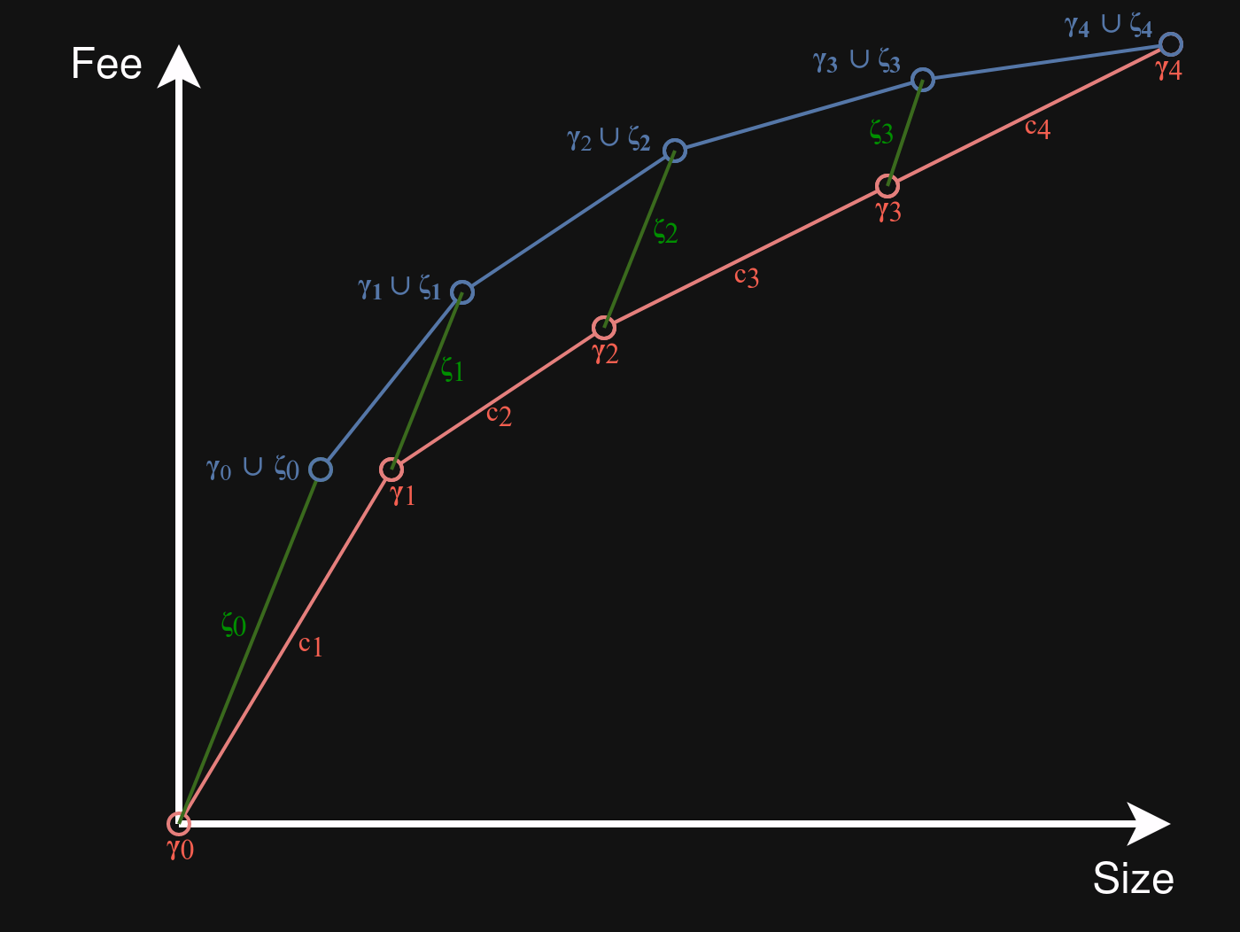
In the drawing below, the blue diagram formed using the \gamma_i+\zeta_i points (plus initial green \zeta_0 segment) is an underestimate for N, the diagram of L_G+L_B. The red diagram shows D, the diagram for L. Intuitively, the blue diagram lies above the red diagram because the slope of all the green lines is never less than that of any red line:
In what follows, we will show that every point on N lies on or above a line making up D. If that holds, it follows that N in its entirety lies on or above D:
The first diagram segment of N, from (0,0) to P(\gamma_0 \cup \zeta_0), is easy: it corresponds to L_G itself, which has feerate (slope) \geq f. All of these points lie on or above the first line of D, from P(\gamma_0) (= (0,0)) to P(\gamma_1), which has feerate (slope) f.
For all other diagram segments of N, we will compare line segments with those in D with the same j = 0 \ldots n-1. In other words, we want to show that the line segment from P(\gamma_j \cup \zeta_j) to P(\gamma_{j+1} \cup \zeta_{j+1}) lies on or above the line through P(\gamma_j) and P(\gamma_{j+1}).
P(\gamma_j \cup \zeta_j) lies on or above the line through P(\gamma_j) and P(\gamma_{j+1}) iff R(\zeta_j) \geq R(c_{j+1}). This follows from R(\zeta_j) \geq f and R(c_{j+1}) \leq f.
P(\gamma_{j+1} \cup \zeta_{j+1}) lies on or above the line through P(\gamma_j) and P(\gamma_{j+1}) iff R(c_{j+1} \cup \zeta_{j+1}) \geq R(c_{j+1}). This follows from the f relations too, except for j=n-1, but there the endpoints of the two graphs just coincide.
All points between P(\gamma_j \cup \zeta_j) and P(\gamma_{j+1} \cup \zeta_{j+1}) lie on or above the line through P(\gamma_j) and P(\gamma_{j+1}), given that the endpoints of the segment do.
Thus, all points on an underestimate of the diagram of L_G + L_B lie on or above the diagram of L, and we conclude that L_G + L_B is a better or equal linearization than L.
Generalization
It is easy to relax the requirement that L_G forms a single chunk. We can instead require that only the lowest chunk feerate of L_G is \geq f. This would add additional points to N corresponding to the chunks of L_G, but they would all lie above the existing first line segment of N, which cannot break the property that N lies on or above D.
Merging individually post-processed linearizations (thus, ones with connected chunks) may result in a linearization whose chunks are disconnected. This means post-processing the merged result can still be useful.
I think the intuition for this is that you’re constructing a (possibly non-optimal) feerate diagram for L_G+L_B by taking the subsets L_G + \sum_{i=1}^j d_i and showing this is a better diagram than that of L. Because you can’t say anything about d_i (the bad parts of each chunk), you’re instead taking the first j chunks as a whole, which have a feerate of f or lower, and then the suffix of L_G that was missed, which has a feerate of f or high, which kinks the diagram up. Kinking the diagram up means this subset has a better diagram than the chunks up to and including c_j.
FWIW, I think this was the argument I was trying to make in my earlier comment but couldn’t quite get a hold of.
I think the general point is just: L^* \ge L if (and only if?) for each \gamma_i (prefixes matching the optimal chunking of L) there exists a set of txs \zeta_i where \gamma_i \cup \zeta_i is a prefix of L^* and R(\zeta_i) \ge R(\gamma_i).
Ah! Actually, isn’t a better “diagram” to consider the ray from the origin to these P(\gamma_i) points in general, ie, for x=0...c_1 plot the y value as R(\gamma_1), for x=c_1..c_2 plot R(\gamma_2) etc. Then (I think) you still compare two diagrams by seeing if all the points on one are below all the points on the other; but have the result that for an optimal chunking, the line is monotonic decreasing, rather than concave.
Also, with that approach, to figure out the diagram for the optimal chunking, you just do the diagram for every tx chunked individually, it’s just f_{opt}(x) = \max(f(x^\prime), x^\prime \ge x).
I think that’s a question of formality. It’s of course obvious that if all points after each chunk lie above the old diagram, then the line from the origin to the first point does too. Yet, we actually do require the property that that line in its entirety lies above the old diagram too. Depending on how “obvious” something needs to be before you choose not to mention it, it could be considered necessary or not.
I don’t think this works. It is very much possible to construct a (fee) graph N that lies above graph D everywhere, but whose derivatives (feerates) aren’t.
EDIT: I see, you’re talking about average feerate for the entire set up to that point, not the feerate of the chunk/section itself. Hmm. Isn’t that just another way of saying the fee diagram is higher?
No, I mean that you can just choose the origin for your first point and go straight to \gamma_1 \cup \zeta_1 when constructing N, and run the same logic.
Yes, precisely – it is another way of saying the same thing, I think it’s just easier to reason about (horizontal line segments that decrease when you’ve found the optimal solution).
Translating the N is better than L proof becomes: look at the feerate at \gamma_i; now consider the feerate for \gamma_i + \zeta_i – it’s higher, because \zeta_i \ge f and the size of that set is greater, and an optimal chunking will extend that feerate leftwards, so N chunks better up to i, for each i, done. You don’t have to deal with line intersections.
Right, that works, we could just drop \gamma_0 \cup \zeta_0 from N. I don’t think it actually simplifies the proof though, because the reasoning for the first segment (now from (0,0) to P(\gamma_1 \cup \zeta_1)), would still be distinct from that for the other segments.
Consider the following:
3 transactions A (fee 0), B (fee 3), C (fee 1), all the same size.
L_1 = [A,B,C], chunked as [AB=3/2, C=1/1]
L_2 = [B,A,C], chunked as [B=3/1, AC=1/2]
L_2 is a strictly better linearization, the fee-size diagram is higher everywhere.
The feerate (using the R(\gamma_i) method) for the middle byte is 3/2 for L_1, but 4/3 for L_2. Would they be considered incomparable by the feerate-size diagram?
Prefix-intersection merging can be simplified to the following:
Given two linearizations L_1 and L_2
(Optionally) Output any prefix of both that’s identical.
Let P_i be the highest-feerate prefix of L_i, for i \in {1,2}.
Assume without loss of generality that R(P_1) \geq R(P_2) (swap the inputs if not).
Let C be the highest-feerate prefix of L_2 \cap P_1.
Output C, remove it from L_1 and L_2, and start over.
So we only need to find the best prefix of the intersection of the highest-feerate prefix with the other linearization, and not the other direction.
This does not break the “as good as both inputs” proof, and from fuzzing it appears it that this doesn’t worsen the result even (it could be that this results in worse results while still being at least as good as both inputs, but that seems not to be the case).
I don’t have a proof (yet) that the algorithms are equivalent, but given that it’s certainly correct still, it’s probably fine to just use this simpler version?
If you have L1=[5,3,1,8,0] (chunk feerates: 5, 4, 0) and L2=[0,8,1,3,5] (chunk feerates: 4, 3) then bestPi chooses C=L2 \cap [5] to start with, ending up as [5,8,3,1,0]. Whereas calculating and comparing C_1 and C_2 would produce [8,5,3,1,0].
But post-processing probably fixes that for most simple examples at least?
(Even if post-processing didn’t fix it; I think so long as merging produces something at least as good as both, that’s fine; quicker/cheaper is more important)
I think you can make post-processing fail to help for this example just by adding a small, low-fee parent transaction P that is a parent to both the 8-fee and 5-fee txs.
I think if you have five transactions, A,B,C,D,E, of 10kvB each at 50,30,10,80,0 sat/vb, and one transaction, P, at 100vB and 0 sat/vb that each of A,D spends an output of, with the same arrangement as above, then post-processing doesn’t fix it either?
Merging isn’t necessarily commutative either, I think, in the case where both linearisations have different (eg, non-overlapping) first chunks at equal feerates.
Hmm, indeed. This example shows that bestPi isn’t always as good as the original PiMerge description.
Given that, I lean towards sticking with the original, as I don’t think that the performance difference between the two is significant. If there was no observable difference at all, it’d make sense to pick the faster one, but that doesn’t seem to be the case now?
The linearizations that come out can differ depending on whether the transactions from L_1 or L_2 is chosen when the found subsets have the same feerate, but I believe this cannot affect the fee-size diagram. Generally I use “smaller size is better” as tie-breaker when comparing equal-feerate chunks, as inside linearization algorithms this sometimes avoids accidentally merging equal-feerate subsets, but I don’t believe it matters here what tie-breaker is chosen. Do you have a counter-example?
EDIT: here is a counterexample:
Transactions: A=1, B=2, C=3, D=2, E=1 (all same size)
L1: [B,E,C,A,D], chunked as [B:2, EC:2, AD:1.5]
L2: [D,B,A,C,E], chunked as [D:2, B:2, AC:2, E:1]
Merge(L1,L2): [B,C,D,E,A], chunked as [BC:2.5, D:2, E:1, A:1]
Merge(L2,L1): [D,B,C,A,E], chunked as [DBC:2.33, A:1, E:1]
Ok, with that counterexample in place I’m now again leaning the other direction: that the right approach is using the simplest algorithm that works.
My impression is that the non-commutativity and non-associativity of merging are effectively randomly stumbled upon through accidentally having/putting transactions in the right order. And these accidents can’t be prevented, and moreover trying more subsets will inevitably mean there is a small chance of finding something better still. However, that doesn’t mean it’s worth spending time on even if it’s a small cost. That time could be better spent on directly trying more things in the linearization algorithm.
Just a quick note, using insights from the composition algorithm, it appears possible to further simplify merging:
Instead of finding the input linearization with the best remaining prefix, it is possible to only consider prefixes of what remains of the original chunks the input linearizations had.
Instead of trying the intersection of that best prefix with every prefix of what remains of the other linearization, it suffices to only consider prefixes aligning with the chunk boundaries of the remainder, or even of just the original chunk boundaries.